Detecting Unstable Electrical Grid With Tinyml

Introduction

Electricity is the heart of modern social and economic development. More and more countries strive to transfer to sustainable energy systems, which is quite a challenging process, as it causes increasingly unstable power generation and grid overloads. The unstable electrical grid can endanger people's lives and the safety of their property. This means that power systems should undergo timely monitoring and optimization, which AI and machine learning can easily handle.

In fact, artificial intelligence has become an essential tool in the power industry. It provides unique self-learning solutions for energy consumption analysis and grid monitoring under dynamically changing circumstances. In this project, we’ll explore how to leverage a machine learning model for efficient monitoring of the electrical grid as shown on the video.

Renewable Energy Sources & Smart EconomyThe ascent of renewable energy sources provide the global community with a much demanded alternative to traditional, finite, and climate-unfriendly fossil fuels. However, their adoption poses a set of new paradigms, the two of which deserve particular attention:

• Prior to the rise of renewable energy sources, the traditional ecosystem involved few production entities (sources) supplying energy to consumers over unidirectional flows. With the advent of renewable options, end-users (households and enterprises) now not only consume energy but have the ability to produce and supply it. Also, for a reliable ecosystem, people need to ensure that energy grids are smarter and equipped with accurate detection of threats and faults.

• Despite the increased flexibility of renewable sources, the management of supply and demand in a more complex generation/distribution/consumption environment and the related economic implications (e.g. the decision to buy energy at a given price or not) have become even more challenging.Need for Grid StabilityIn a smart grid, consumer demand information is collected, and centrally evaluated against current supply conditions. The resulting proposed price information is sent back to customers for them to make decisions about further usage. As the whole process is time-dependent, dynamic estimation of grid stability becomes not only a concern but a major requirement.

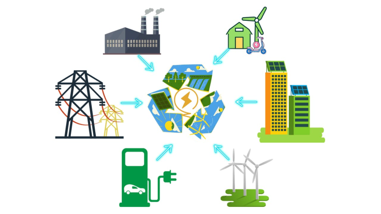
Put simply, the objective is to understand and plan for both energy production and/or consumption disturbances and fluctuations introduced by system participants in a dynamic way, taking into consideration not only technical aspects but also how participants respond to changes in the associated economic aspects (energy costs).

The Challenges of Applying AI to Smart Electric Grids

• Insufficient data accumulation: there aren’t enough data samples that meet the requirements of diverse AI technology applications, and sample collection can be a time-consuming process.
• Reliability: although AI technology applied to power systems demonstrates high levels of problem identification, it doesn’t always meet the requirements of practical application.
• Infrastructure: applying AI is based on abundant data samples, advanced computing power, and distributed communication collaboration. However, the supporting capacity and level of relevant infrastructure resources such as quick production AI algorithms, and distributed collaboration platforms need improvement.
• Lack of power industry-specific algorithms: compared to perception, prediction, and security maintenance, algorithm adaptability of AI in power systems is still weak.

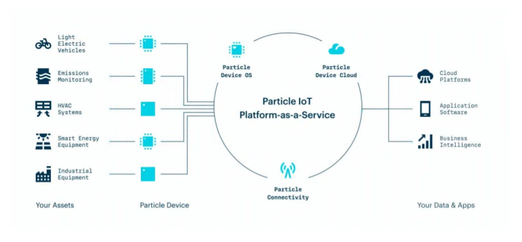
In this project, we will explore how we can predict electric grid stability with a free platform, Neuton TinyML, and an integrated IoT Platform-as-a-Service, Particle IoT that helps to deploy software applications to connected devices, from edge to cloud and back.

Also, we will explore the communication infrastructure for such electric grid operations. With the combined knowledge of AI and IoT, we will try to solve some parts of the above-mentioned challenges.

The original dataset contains 10, 000 observations. It also contains 12 primary predictive features and two dependent variables.

Predictive features:

• 'tau1' to 'tau4': the reaction time of each network participant, a real value within the range 0.5 to 10 ('tau1' corresponds to the supplier node, 'tau2' to 'tau4' to the consumer nodes);
• 'p1' to 'p4': nominal power produced (positive) or consumed (negative) by each network participant, a real value within the range -2.0 to -0.5 for consumers ('p2' to 'p4'). As the total power consumed equals the total power generated, p1 (supplier node) = - (p2 + p3 + p4);
• 'g1' to 'g4': price elasticity coefficient for each network participant, a real value within the range 0.05 to 1.00 ('g1' corresponds to the supplier node, 'g2' to 'g4' to the consumer nodes; 'g' stands for 'gamma');

Dependent variables:

• 'stab': the maximum real part of the characteristic differentia equation root (if positive, the system is linearly unstable; if negative, linearly stable);
• 'stabf': a categorical (binary) label ('stable' or 'unstable').

As there is a direct relationship between 'stab' and 'stabf', 'stab' will be dropped and 'stabf' will remain as the sole dependent variable. Here is the link to the dataset: https://archive.ics.uci.edu/ml/datasets/Electrical+Grid+Stability+Simulated+Data+

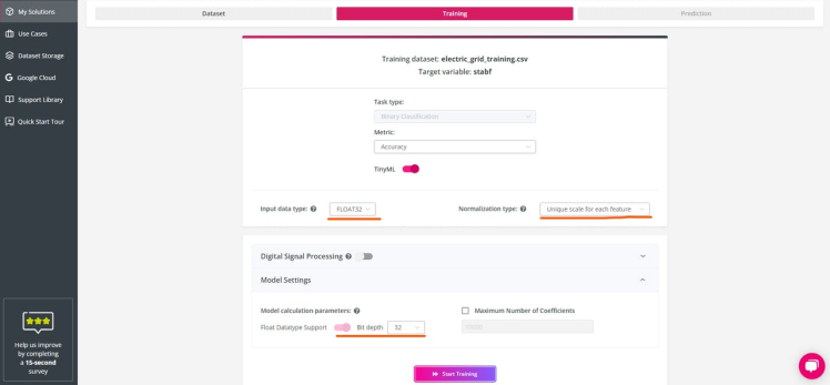
On the Neuton platform, we will upload the dataset for our use case and select 'stabf' as the target variable.

In the training parameters, set the Input data type FLOAT32 andNormalization type "Unique scale for each feature". Then proceed to model training.

Step 2: Training and Exploratory Data Analysis

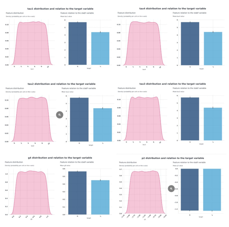
Once the training has started, we see the model data analysis which helps us to understand the close relationship between the original dependent and independent variables.

Correlation:

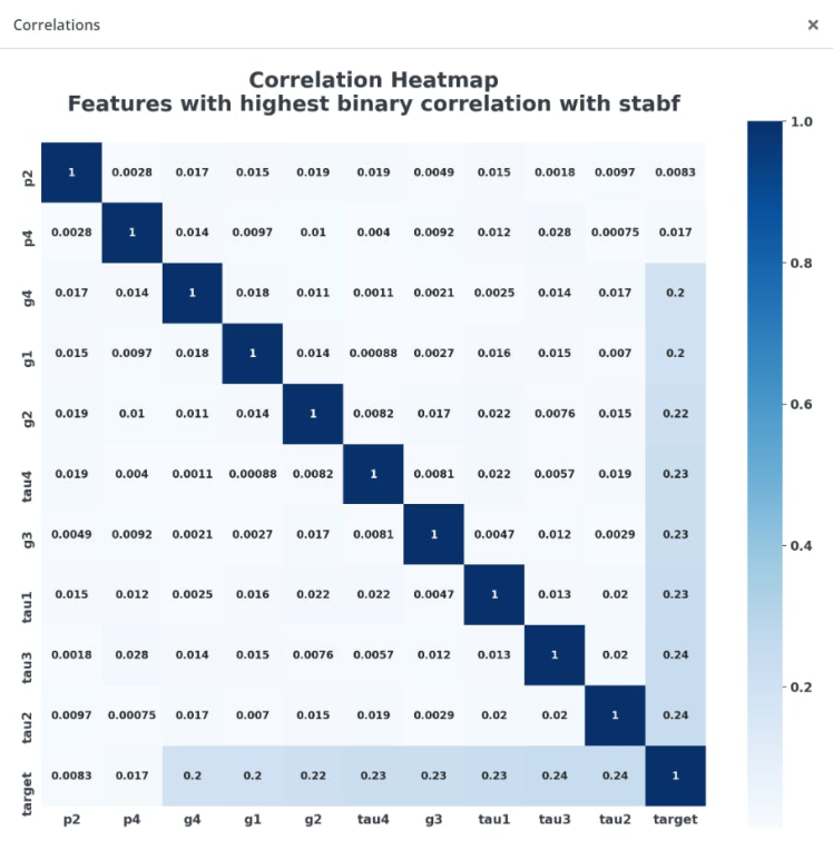
It is important to verify the correlation between each numerical feature and the dependent variable, as well as the correlation among numerical features leading to potential undesired collinearity. The heatmap below provides an overview of the correlation between the dependent variable ('stabf' or 'target') and the top 10 numerical features with the highest binary correlation to the target.

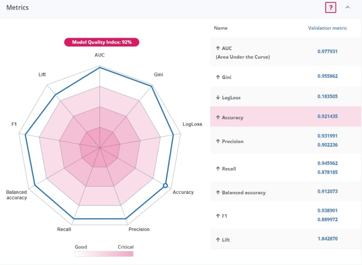
After the training is over, we can see the model metrics: the model accuracy is 0.921435!

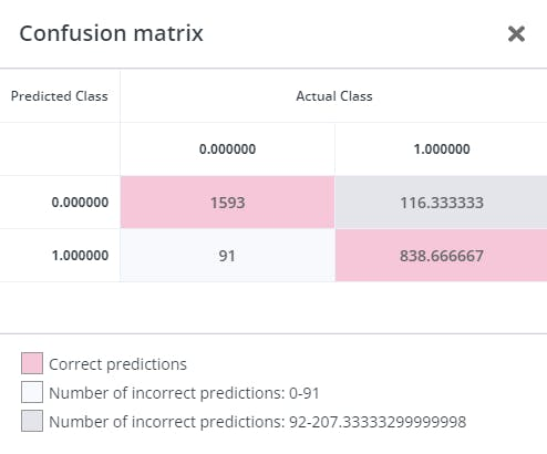
We can also see the classification performance using the generated confusion matrix.

Download the model for further deployment on our IoT device.

We have selected the Particle Argon board for this project (although you can use any Particle board without the need to reprogram each board). The Particle Argon is a powerful Wi-Fi development kit that you can use on Wi-Fi networks.

Equipped with the Nordic nRF52840 and Espressif ESP32 processors, the Argon has built-in battery charging circuitry which makes it easier to connect a Li-Po battery and 20 mixed-signal GPIOs to interface with sensors, actuators, and other electronics.

Particle IoT boards are secure and fully equipped to allow Smart Grid Infrastructure to deliver data and updates on grid failures at a faster and cheaper rate.

Setting up Particle IDEand Workbench:

Add your downloaded Neuton model inside the Particle Workbench project folder. Your folder structure will look like this (checksum, parser, protocol, application and StatFunctions) These files are required to make predictions on data received over serial communication using the CSV uploader tool.

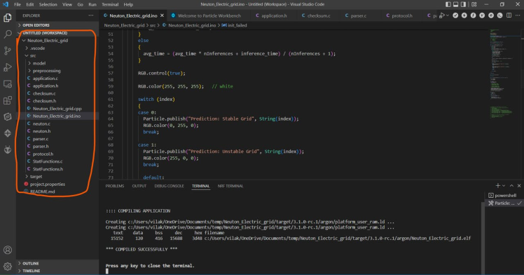
Here is the most important function:

static float* on_dataset_sample(float* inputs)
{
 if (neuton_model_set_inputs(inputs) == 0)
  {
 uint16_t index;
 float* outputs;

 uint64_t start = micros();
 if (neuton_model_run_inference(&index, &outputs) == 0)
    {
 uint64_t stop = micros();

 uint64_t inference_time = stop - start;
 if (inference_time > max_time)
        max_time = inference_time;
 if (inference_time < min_time)
        min_time = inference_time;

 static uint64_t nInferences = 0;
 if (nInferences++ == 0)
      {
        avg_time = inference_time;
      }

else
      {
        avg_time = (avg_time * nInferences + inference_time) / (nInferences + 1);
      }

      RGB.control(true);

      RGB.color(255, 255, 255);   // white

 switch (index)
      {
 case 0:      
        Particle.publish("Prediction: Stable Grid", String(index));
        RGB.color(0, 255, 0);
 break;

 case 1:
        Particle.publish("Prediction: Unstable Grid", String(index));
        RGB.color(255, 0, 0);
 break;

 default:
 break;
      }

 return outputs;
    }
  }

 return NULL;
}

Compile the application in the cloud or locally. Once compiled, you are ready to flash it to your device. Make sure you have selected the correct Particle OS for your device.


CSV data upload utility:

We are going to test our predictions by sending the test data features from our test dataset CSV file over a USB serial port.

• Install dependencies,

# For Ubuntu
$ sudo apt install libuv1-dev gengetopt
# For macOS
$ brew install libuv gengetopt

• Clone this repo,

$ git clone https://github.com/Neuton-tinyML/dataset-uploader.git
$ cd dataset-uploader

• Run “make” to build the binaries,

$ make

Once it's done, you can send the CSV file over USB.

$./uploader -s /dev/ttyACM0 -b 230400 -d /home/vil/Desktop/electric_grid_test.csv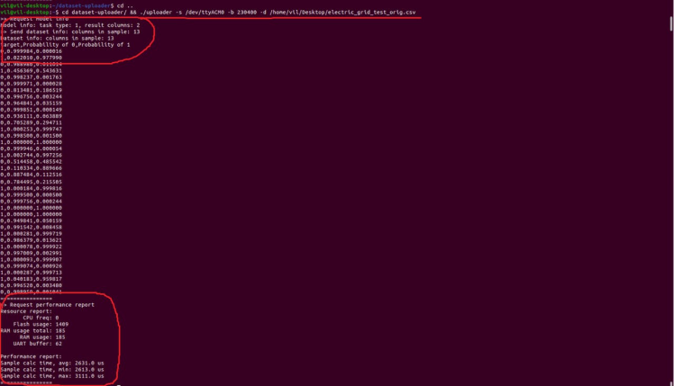

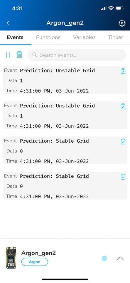
The prediction is printed on the Particle IoT cloud.

Monitoring the stability of the electrical grid helps to reveal "unreliable" energy sources and avoid serious damage. The best strategy for such AI+IoT projects is not only making predictions but also collecting and reporting data in order to improve models for future devices like Particle and make OTA updates easier.